
Archivo:Savitzky-golay pic gaussien bruite.svg

Tamaño de esta previsualización PNG del archivo SVG: 610 × 407 píxeles. Otras resoluciones: 320 × 214 píxeles · 640 × 427 píxeles · 1024 × 683 píxeles · 1280 × 854 píxeles · 2560 × 1708 píxeles.
Ver la imagen en su resolución original ((Imagen SVG, nominalmente 610 × 407 pixels, tamaño de archivo: 43 kB))
Resumen
| Descripción |
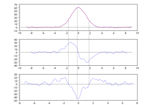
English: Savitzky-Golay algorithm (3rd degree polynomial, 9 points) applied on a gaussian peak with random noise: smoothing (top), first derivation (middle), second derivation (bottom).
The dashed lines highlight the zeros of the second dérivative (inflection points of the peak) and its minimum (top of the peak). Created with Scilab, processed with Inkscape.Français : Application de l'algorithme de Savitzky-Golay sur un pic gaussien bruité (polynôme de degré 3, 9 points) : lissage (haut), dérivée (milieu), dérivée seconde (bas).
Les traits pointillés mettent en évidence l'annulation de la dérivée seconde (points d'inflexion du pic) et son minimum (sommet du pic). Créé avec Scilab, retravaillé avec Inkscape. |
| Fecha | |
| Fuente | Trabajo propio |
| Autor | Christophe Dang Ngoc Chan |
| SVG desarrollo |  English: English version by default.
Français : Version française, si les préférences de votre compte sont réglées (voir Special:Preferences). El código fuente de esta imagen SVG es válido. Este gráfico vectorial fue creado con Scilab This file uses embedded text. |
| Código fuente | (1) File generateur_pic_bruit.sce : generates a set of data and save it in the file noisy_gaussian_peak.txt.
SciLab code// **********
// Constants and initialisation
// **********
clear;
chdir("mypath/");
// parameters of the noisy curve
paramgauss(1) = 60; // height of the gaussian curve
paramgauss(2) = 3; // "width" of the gaussian curve
var=0.01; // variance of the noise normal law
nbpts = 100 // nombre of points
halfwidth = 3*paramgauss(2) // range for x
step = 2*halfwidth/nbpts;
// **********
// Fonctions
// **********
// gaussian peak
function [y] = gauss(A, x)
// A(1) : height of the peak
// A(2) : "width" of the peak
y = A(1)*exp(-x.^2/A(2));
endfunction
// **********
// Main program
// **********
// Generation of data
for i=1:nbpts
x = step*i - halfwidth;
X(i) = x;
Y(i) = gauss([paramgauss], x) + rand(var, "normal");
end
// Saving the data
write ("noisy_gaussian_peak.txt", [X, Y])
(2) File savitzkygolay.sce : processes the data.
Data// **********
// Constants and initialisation
// **********
clear;
clf;
chdir("mypath/")
// smoothing parameters :
width = 9; // width of the sliding window (number of pts)
poldeg = 3; // degree of the polynomial
// **********
// Functions
// **********
// Convolution coefficients
function [a]=convolcoefs(m, d)
// m : width of the window (number of pts)
// d : degree of the polynomial
l = (m-1)/2; // half-width of the window
z = (-l:l)'; // standardised abscissa
J = ones(m,d+1);
for i = 2:d+1
J(:,i) = z.^(i-1); // jacobian matrix
end
A = (J'*J)^(-1)*J';
a = A(1:3,:);
endfunction
// smoothing, determination of the first and second derivatives
function [y, yprime, ysecond] = savitzkygolay(X, Y, width, deg)
// X, Y: collection of data
// width: width of the window (number of pts)
// deg: degree of the polynomial
n = size(X, "*");
l = floor(width/2);
step = (X($)-X(1))/(n - 1);
y = Y;
yprime=zeros(Y);
ysecond=yprime;
a = convolcoefs(width, deg);
a(2,:) = 1/step*a(2,:);
a(3,:) = 2/step^2*a(2,:);
for i = 1:width
Ymat(i, :) = Y(i: n-width+i)';
end
solution = a*Ymat;
y = solution(1, :)';
yprime = solution(2, :)';
ysecond = solution(3, :)';
endfunction
// **********
// Main program
// **********
// data reading
data = read("noisy_gaussian_peak.txt", -1, 2)
Xinit = data(:,1);
Yinit = data(:,2);
//subplot(3,1,1)
//plot(Xdef, Ydef, "b")
// Data processing
[Ysmooth, Yprime, Ysecond] = savitzkygolay(Xinit, Yinit, width, poldeg);
// Display
offset = floor(width/2);
nbpts = size(Xinit, "*");
X1 = Xinit((offset+1):(nbpts-offset)); // removal of non-smotthed points
subplot(3,1,1)
plot(Xinit, Yinit, "b")
plot(X1, Ysmooth, "r")
subplot(3,1,2)
plot(X1, Yprime, "b")
subplot(3,1,3)
plot(X1, Ysecond, "b")
(3) When the sampling step is not constant, i.e. xi - xi - 1 varies, then it is possible to determine the polynomial by multi-linear regression. Text// **********
// Constants and initialisation
// **********
clear;
clf;
chdir("mypath\")
// smoothing parameters
width = 9; // width of the sliding window (number of pts)
// **********
// Functions
// **********
// 3rd degree polynomial
function [y]=poldegthree(A, x)
// Horner method
y = ((A(1).*x + A(2)).*x + A(3)).*x + A(4);
endfunction
// regression with the 3rd degree polynomial
function [A]=regression(X, Y)
// X, Y: column vectors of "width" values ;
// determines the polynomial of degree 3
// a*x^2 + b*x^2 + c*x + d
// by regression on (X, Y)
XX = [X.^3; X.^2; X];
[a, b, sigma] = reglin(XX, Y);
A = [a, b];
endfunction
// smoothing, determination of the first and second derivatives
function [y, yprime, ysecond] = savitzkygolay(X, Y, larg)
// X, Y: collection of data
n = size(X, "*");
l = floor(larg/2); // halfwidth
y=Y;
yprime=zeros(Y);
ysecond=yprime;
for i=(l+1):(n-l)
intervX = X((i-l):(i+l),1);
intervY = Y((i-l):(i+l),1);
Aopt = regression(intervX', intervY');
x = X(i);
y(i) = poldegthree(Aopt,x);
// Yfoo=poldegthree(Aopt,intervX);
// subplot(3,1,1) ; plot(intervX, Yfoo, "r")
yprime(i) = (3*Aopt(1)*x + 2*Aopt(2))*x + Aopt(3); // Horner
ysecond(i) = 6*Aopt(1)*x + 2*Aopt(2);
end
endfunction
// **********
// Main program
// **********
// data reading
data = read("noisy_gaussian_peak.txt", -1, 2)
Xinit = data(:,1);
Yinit = data(:,2);
//subplot(3,1,1)
//plot(Xdef, Ydef, "b")
// Data processing
[Ysmooth, Yprime, Ysecond] = savitzkygolay(Xinit, Yinit, width);
// Display
offset = floor(width/2);
nbpts = size(Xinit, "*");
vector1 = (offset+1):(nbpts-offset); // suppresion des points non-lissés
X1 = Xinit(vector1);
Y0 = Yliss(vector1)
Y1 = Yprime(vector1);
Y2 = Ysecond(vector1);
subplot(3,1,1)
plot(Xinit, Yinit, "b")
plot(X1, Y0, "r")
subplot(3,1,2)
plot(X1, Y1, "b")
subplot(3,1,3)
plot(X1, Y2, "b")
|
Licencia
Yo, titular de los derechos de autor de esta obra, la publico en los términos de las siguientes licencias:

|
Se autoriza la copia, distribución y modificación de este documento bajo los términos de la licencia de documentación libre GNU, versión 1.2 o cualquier otra que posteriormente publique la Fundación para el Software Libre; sin secciones invariables, textos de portada, ni textos de contraportada. Se incluye una copia de la dicha licencia en la sección titulada Licencia de Documentación Libre GNU. |
Este archivo se encuentra bajo la licencia Creative Commons Attribution-Share Alike 3.0 Unported, 2.5 Generic, 2.0 Generic and 1.0 Generic
- Eres libre:
- de compartir – de copiar, distribuir y transmitir el trabajo
- de remezclar – de adaptar el trabajo
- Bajo las siguientes condiciones:
- atribución – Debes otorgar el crédito correspondiente, proporcionar un enlace a la licencia e indicar si realizaste algún cambio. Puedes hacerlo de cualquier manera razonable pero no de manera que sugiera que el licenciante te respalda a ti o al uso que hagas del trabajo.
- compartir igual – En caso de mezclar, transformar o modificar este trabajo, deberás distribuir el trabajo resultante bajo la misma licencia o una compatible como el original.
Puedes usar la licencia que prefieras.
Historial del archivo
Haz clic sobre una fecha y hora para ver el archivo tal como apareció en ese momento.
| Fecha y hora | Miniatura | Dimensiones | Usuario | Comentario | |
|---|---|---|---|---|---|
| actual | 13:07 9 nov 2012 | | 610 × 407 (43 kB) | Cdang | dashed line to highlight the inimum of the second derivative |
| 10:50 9 nov 2012 |  | 610 × 407 (43 kB) | Cdang | {{Information | description = {{en|1=Savitzky-Golay algorithm (3<sup>rd</sup> degree polynomial, 9 points) applied on a gaussian peak with random noise: smoothing (top), first derivation (middle), second derivation (bottom). Created with Scilab, proce... |
Usos del archivo
La siguiente página usa este archivo:
Uso global del archivo
Las wikis siguientes utilizan este archivo:
- Uso en fr.wikipedia.org
- Uso en fr.wikibooks.org
- Uso en nl.wikipedia.org